|
PIPS-IPM++ Solver and Tools
a parallel interior-point method for doubly bordered block diagonal linear programs
|
|
PIPS-IPM++ Solver and Tools
a parallel interior-point method for doubly bordered block diagonal linear programs
|
The gmspips executable of PIPS-IPM++ expects as input the data of LP (BlockLP), separated by blocks \(0, \ldots, N\). That is, \(N+1\) files that contain the matrices \(T_i\), \(W_i\), \(F_i\) and vectors \(c_i\), \(h_i\) need to be provided, using a format and naming convention that is understood by gmspips. The expected format is the GAMS Data Exchange Format (GDX), which allows to store these matrices, vectors, and corresponding equation and variables names in a compact form that can be efficiently processed. The conventions used for naming the matrices and vectors in the GDX files are, however, derived from conventions used by GAMS tools like GAMS/Convert.
With gmschk, a tool exists that takes as input a GDX file with the data of a full LP and assignments of variables and equations to blocks, and outputs \(N+1\) GDX files with the data for each block separately. In addition, tools are available to generate the input GDX file for gmschk, e.g., by using MPS2GMS to convert an LP given in .lp or MPS format and block assignments given as DEC files to a GDX file.
In the following, we describe how to (manually) annotate a GAMS model to provide block structure information suitable for PIPS-IPM++, how to generate the input file for gmschk, how to run PIPS-IPM++ from GAMS, and how to read a solution file from gmspips back into GAMS. The initial content for this section has been taken from Chapter 4.3 of [11].
For a model with linking variables and linking constraints that has \(N\) blocks of non-linking variables, the annotation scheme utilizes the .stage attribute of GAMS variables and equations and can be summarized as follows:
Variables:
Equations:
When considering the block-diagonal structure (BlockLP), the stage annotation is given by
\begin{align}\text{min} \quad & c_0^T x_0 & + & c_1^T x_1 & + & c_2^T x_2 & \cdots\; & + c_N^T x_N \\ \text{s.t.} \quad & T_0 x_0 & & && & & & =\; & h_0 && \left.\right\} \text{stage 1}\\ & T_1 x_0 & + & W_1 x_1 && & & & =\; & h_1 && \left.\right\} \text{stage 2}\\ & T_2 x_0 & & & + & W_2 x_2 & & & =\; & h_2 && \left.\right\} \text{stage 3}\\ & \vdots & & && & \ddots\; & & & \vdots \\ & T_N x_0 & & && & & + W_N x_N & =\; & h_N && \left.\right\} \text{stage N+1}\\ & F_0 x_0 & + & F_1 x_1 & + & F_2 x_2 & \cdots\; & + F_N x_N & =\; & h_{N+1}, && \left.\right\} \text{stage N+2} \\ & \underbrace{\qquad}_{\text{stage 1}} & & \underbrace{\qquad}_{\text{stage 2}} & & \underbrace{\qquad}_{\text{stage 3}} & & \quad\underbrace{\qquad\;\;}_{\text{stage N+1}} \end{align}
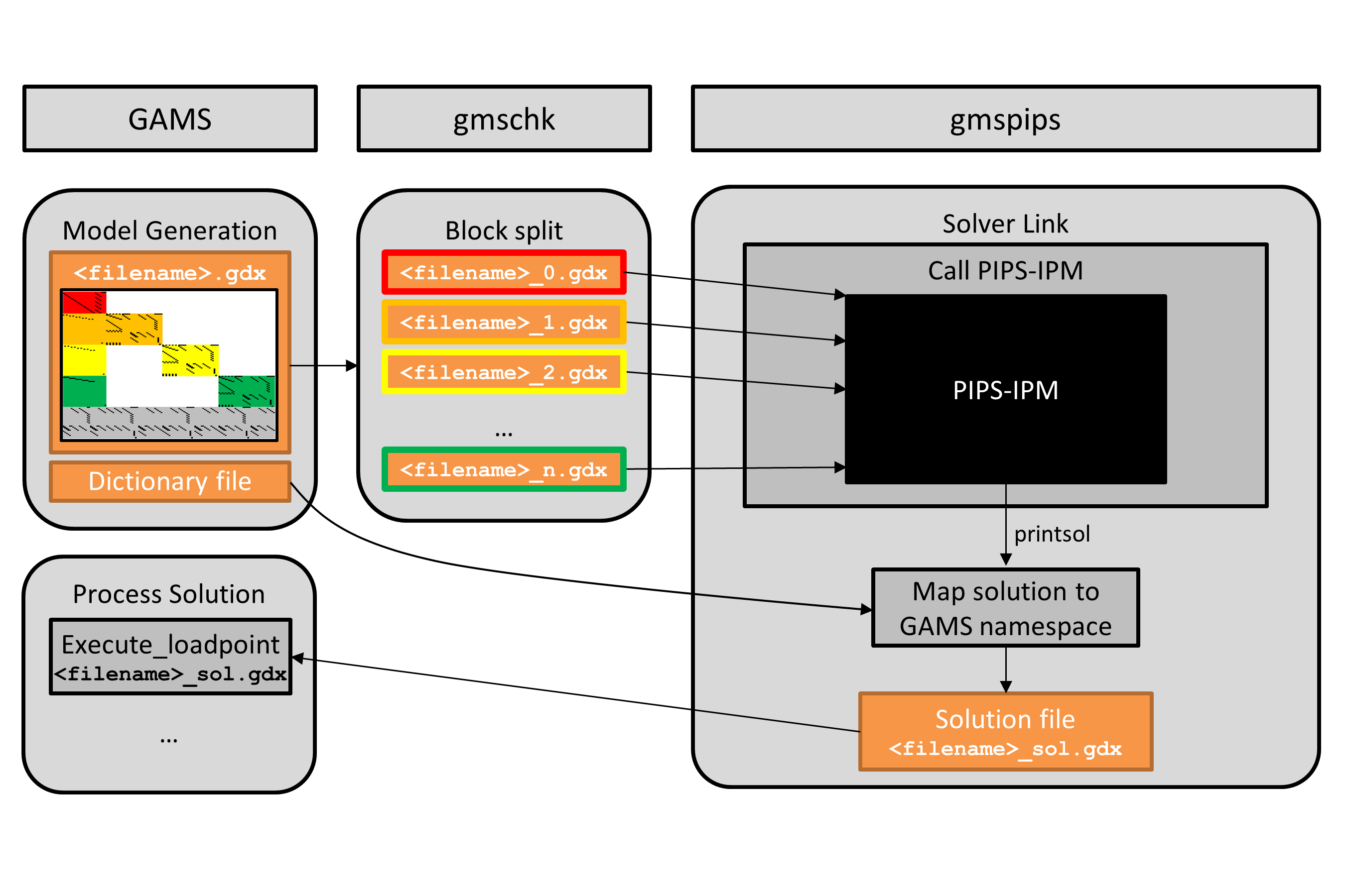
Once a model has been annotated, a corresponding model instance can be generated in a format that fits the requirements of PIPS-IPM++ and the GDX/PIPS-IPM++ link (gmspips), in particular. That process is called model generation.
A model with \(N\) blocks of non-linking variables is represented by \(N+1\) GDX files that hold all the required information about the block structured problem. However, first one large "all-in-one" GDX file that contains the entire problem information including the user's annotation of the block structure has to be generated (experiments that generate the \(N+1\) GDX files directly were conducted, see Section 4.3.3.3 of [11], but corresponding code is not available in publicly available versions of GAMS and PIPS-IPM++). The "all-in-one" GDX file can then be split into the required \(N+1\) GDX files with the gmschk tool.
To generate the all-in-one GDX file, let's call it blockAll.gdx, the following steps need to be taken:
$echo jacobian blockAll.gdx > convert.opt
If the GDX file blockAll.gdx has been created successfully, it needs to be split into several block files. The tool gmschk checks for consistency of the annotation and can also be used to split such a file. To split blockAll.gdx into \(N+1\) GDX files as required by PIPS-IPM++, run gmschk for example as follows
/path/to/gmschk -T N+1 blockAll.gdx
Note that N+1 must be replaced by the proper number that represents the number of (variable) blocks of the model instance at hand. As a result, \(N+1\) GDX files called blockall0.gdx, blockall1.gdx, ..., blockallN.gdx are created.
For large-scale instances, generating the "all-in-one" GDX file can require significant time and memory resources. Efficiency of this stop can be improved by omitting information in the GDX file that is not always necessary.
The CONVERT options file should contain the instruction to write a GDX version with the LP data. If the string noVEnames is added to the filename, original equation and variable names are suppressed. This can be useful for the further processing of the GDX files, especially for large model instances. While having the original equation and variable names available in PIPS-IPM++ can be useful for debugging purposes, they are not necessary for the solving process and can make the GDX file significantly larger and slow to write and read. The solver option file convert.opt could for example look as follows:
jacobian fileName_noVEnames.gdx
To further reduce the size of the GDX file and to improve performance of writing the GDX file, the string noUELs can be added to the file name. This results in unique elements (UELs) not being written to the GDX file. In GAMS jargon, a "UEL", also known as "label", refers to the elements of one-dimensional sets, a fundamental data structure in GAMS. The solver option file convert.opt could for example look as follows:
jacobian fileName_noVEnames_noUELs.gdx
Model instances captured in GDX files created without UELs can still be split with gmschk, solved with PIPS-IPM++, and also the solution reporting works.
To import the solution from PIPS-IPM++ back to GAMS, the following steps are required.
After generating the model, a dictionary file that holds information about the variable and equation names of the GAMS model needs to be saved. By default this dictionary file is created in the process directory (225a, 225b, ...) of the current GAMS run. The process directory is temporary and by default it gets deleted after a (successful) GAMS run. Hence, it is recommended to retrieve the dictionary file via system call
execute 'mv -f %gams.scrdir%gamsdict.dat <filename>_dict.gdx';
This moves the dictionary out of the process directory into the working directory. Note that <filename> has to correspond to the name of the GDX file created by CONVERT.
execute_loadpoint '<filename>_sol.gdx';
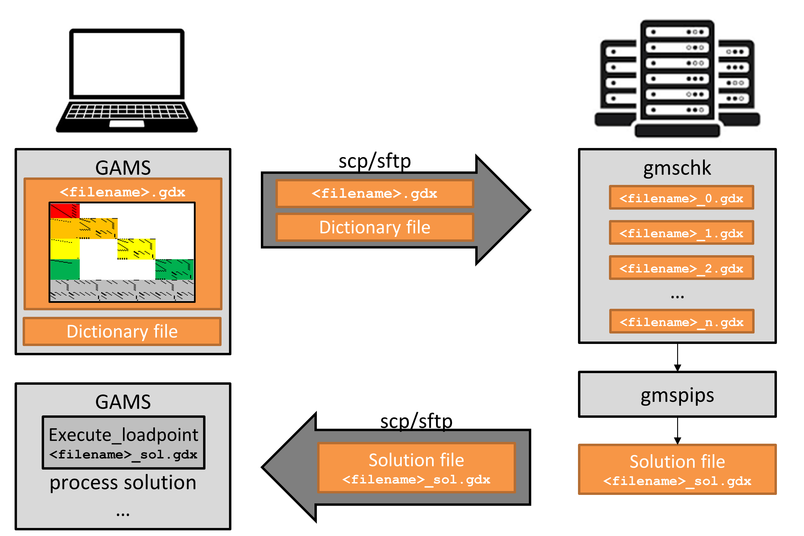
The entire workflow can be visualized as follows:
The workflow is also summarized in the following code snippet, where the number of tasks and the number of blocks is assumed to be computed and stored in compile time variables NBTASKS% and NBBLOCKS%.
A few limitations are worthwhile to mention:
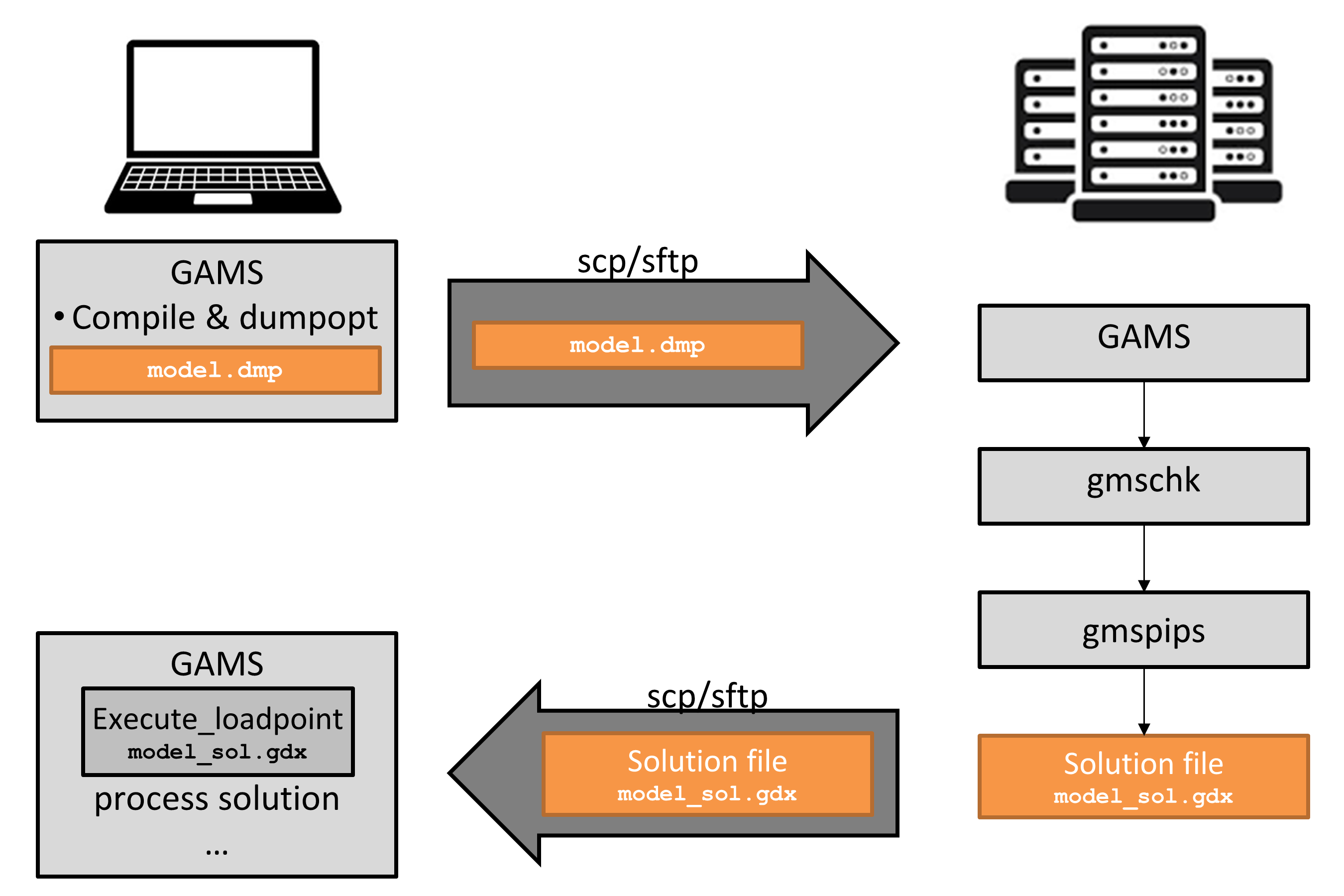
In some situations, it can be useful to use different machines for the instantiation of a model and the solution of the model instance, for example, when the model instantiation needs to pull data out of various sources (e.g., MS Excel), and the solution should run on a dedicated HPC (High Performance Computing) system. This section discusses ways to handle such platform dependencies and to carry out certain steps of the GAMS/PIPS-IPM++ work flow on different machines.
If the modeler has a local machine available that has sufficient resources to generate the model instance, then the resulting "all-in-one" GDX file can be transferred to the HPC system, where it is split into \(N+1\) GDX files and PIPS-IPM++ is called. If needed, the solution file can be transferred back to the local machine once gmspips has terminated.
If resources on the locally available machine are insufficient to execute the GAMS program, the so-called dump file is a convenient way to capture an instance with its associated data and algebraic model representation on the local machine, but to generate the actual LP instance on a different machine. To do so, add dumpopt=11 to the list of command line parameters when running GAMS. To create the dump file, it suffices to compile but not execute a GAMS program. This can be accomplished by instructing GAMS to compile only via command line parameter action=c. An exemplary command line call of GAMS to create a dump file model.dmp in compile only mode looks as follows:
gams model.gms action=c dumpopt=11
The file model.dmp can then be transferred to a suitable machine and can be executed by GAMS via
gams model.dmp
Sometimes, the execution of dump files may not work right away, for example, because output files (e.g., when the put writing facility or commands like execute_unload are used) should be created in particular locations, assuming a certain directory structure that only exists on the local machine that was used to create the dump file. Those errors can usually be fixed or ignored easily.